Who does the best triple axel?
To recap, the first post in this series set out the overall project: to predict grade-of-execution scores in international singles figure skating competions, using data from the website skatingscores. Ideally we’d like to be able to answer high-level questions involving the relative difficulty of different elements and the abilities of the skaters. The second post showed how to scrape the data.
This post will start to analyse the data by fitting a relatively simple model to a relatively homogenous subset of the data - the scores for triple axel jumps. The triple axel seemed like a good choice for a first analysis because it is attempted by most of the top skaters, but is difficult enough that even the best skaters can’t be 100% sure of pulling it off.
You can find all the code I used for this analysis here.
Data
The data that we fetched in the first post come from the 2019/2020 grand prix series, the 2020 Four Continents Championships, the 2020 European championships and the 2020 Japanese, Russian and US national championships.
Of these we will look only at 3A elements with no deductions for
under-rotation. Altogether the data records 305 qualifying triple axels,
attempted by 108 different skaters and receiving 2687 scores.
The reason for excluding jumps with a rotation deduction is that in these cases the judges' scores are not supposed to reflect how well the jump was executed compared to other triple axels, but to other under-rotated triple axels.
Project structure
Since the data has a quite specific and informative structure that needs to be taken into account, I was pretty sure that I wanted to try a custom Stan model. I recently wrote a cookiecutter template for just this kind of project, so I thought I’d try it out and hopefully save writing a bit of boilerplate code.
To set up the project I set up a new virtual environment and installed cookiecutter in it:
$ python -m venv ~/.venvs/figure_skating
tedgro@nnfcb-l0601 ~/Code
$ source ~/.venvs/figure_skating/bin/activate
(figure_skating) tedgro@nnfcb-l0601 ~/Code
$ pip install cookiecutter
Next I used the cookiecutter command to download the template from github and
start a questionnaire:
...
(figure_skating) tedgro@nnfcb-l0601 ~/Code
$ cookiecutter gh:teddygroves/cookiecutter-cmdstanpy
You've downloaded /Users/tedgro/.cookiecutters/cookiecutter-cmdstanpy before. Is it okay to delete and re-download it? [yes]:
project_name [project_name]: Figure skating
repo_name [figure_skating]:
author_name [Your name (or your organization/company/team)]: Teddy Groves
description [A short description of the project.]: Statistical models of figure skating data
Select open_source_license:
1 - MIT
2 - BSD-3-Clause
3 - No license file
Choose from 1, 2, 3 [1]: 1
I now had a folder called figure_skating with the following structure:
(figure_skating) tedgro@nnfcb-l0601 ~/Code
$ tree figure_skating
figure_skating
├── LICENSE
├── Makefile
├── README.md
├── bibliography.bib
├── data
│   ├── fake
│   │   └── readme.md
│   ├── prepared
│   │   └── readme.md
│   └── raw
│       ├── raw_measurements.csv
│       └── readme.md
├── fit_fake_data.py
├── fit_real_data.py
├── prepare_data.py
├── report.md
├── requirements.txt
├── results
│   ├── infd
│   │   └── readme.md
│   ├── input_data_json
│   │   └── readme.md
│   ├── loo
│   │   └── readme.md
│   ├── plots
│   │   └── readme.md
│   └── samples
│       └── readme.md
└── src
    ├── cmdstanpy_to_arviz.py
    ├── data_preparation.py
    ├── fake_data_generation.py
    ├── fitting.py
    ├── model_configuration.py
    ├── model_configurations_to_try.py
    ├── pandas_to_cmdstanpy.py
    ├── readme.md
    ├── stan
    │   ├── custom_functions.stan
    │   ├── model.stan
    │   └── readme.md
    └── util.py

12 directories, 30 files
I moved the fetch_scores.py script and the resulting csv file scores.csv
into the this folder.
First model
The first model I wanted to try was a basic hierarchical ordered logistic regression:
\begin{align*} score &\sim ordered\ logistic(ability, cutpoints)\newline ability &\sim normal(\mu, 1)\newline \mu &\sim normal(0, 1)\newline cutpoints_5 &= 0\newline cutpoints_{2:11} - cutpoints_{1:10} &\sim normal(0.2, 0.3) \end{align*}
I expected that this model would be too simple, as it is missing the rather important information that a lot of the scores come from the exact same jumps. However I think it is generally good practice not to include this kind of detail, and add it to a simpler model when there is a clear benefit from doing so.
To implement this model in Stan I first added the following function to the
file custom_functions.stan. The purpose of the function is to get a vector of
cutpoints from a vector of differences while ensuring that a certain cutpoint
is exactly zero, which should make the model parameters easier to interpret and
the priors easier to specify.
vector get_ordered_from_diffs(vector diffs, int fixed_ix, real fixed_val){
  /* Get an ordered vector of length K from a vector of K-1 differences, plus
     the index of an entry that is exactly fixed_val.
  */
  int K = rows(diffs) + 1;
  vector[K] out;
  out[fixed_ix] = fixed_val;
  out[1:fixed_ix-1] = reverse(-cumulative_sum(reverse(diffs[1:fixed_ix-1])));
  out[fixed_ix+1:K] = cumulative_sum(diffs[fixed_ix:K]);
  return out;
}
The rest of the model as follows:
functions {
#include custom_functions.stan
}
data {
  int<lower=1> N;
  int<lower=1> N_skater;
  int<lower=1> N_grade;
  int<lower=1,upper=N_skater> skater[N];
  int<lower=1,upper=N_grade> y[N];
  int<lower=1> N_test;
  int<lower=1,upper=N_skater> skater_test[N_test];
  int<lower=1,upper=N_grade> y_test[N_test];
  int<lower=0,upper=1> likelihood;
  vector[2] prior_mu;
  vector[2] prior_cutpoint_diffs;
}
parameters {
  real mu;
  vector[N_skater] ability;
  vector<lower=0>[N_grade-2] cutpoint_diffs;
}
transformed parameters {
  ordered[N_grade-1] cutpoints = get_ordered_from_diffs(cutpoint_diffs, 5, 0);
}
model {
  mu ~ normal(prior_mu[1], prior_mu[2]);
  ability ~ normal(0, 1);
  cutpoint_diffs ~ normal(prior_cutpoint_diffs[1], prior_cutpoint_diffs[2]);
  if (likelihood){
    y ~ ordered_logistic(mu + ability[skater], cutpoints);
  }
}
generated quantities {
  vector[N_test] yrep;
  vector[N_test] llik;
  for (n in 1:N_test){
    real eta = mu + ability[skater_test[n]];
    yrep[n] = ordered_logistic_rng(eta, cutpoints);
    llik[n] = ordered_logistic_lpmf(y_test[n] | eta, cutpoints);
  }
}
Fitting fake data
After customising the python functions to match my model I filtered the data
with the prepare_data.py script, then generated some fake scores and fit the
model to them in priors only and likelihood-included mode using the
fit_fake_data.py script. Posterior samples appeared fairly quickly and
without diagnostic warnings in both cases and the loo comparison looked ok too:
Loo comparison:
                                           rank          loo        p_loo ...         se        dse  warning
sim_study-20210322170324-simple_posterior     0 -4952.580176    93.164296 ...  32.849310   0.000000    False
sim_study-20210322170324-simple_prior         1 -7919.559170  2448.849177 ...  47.280981  44.640614     True
I wasn’t too worried about the loo warning for the prior model. To check that it wasn’t too far wrong I wrote some sanity-checking plotting functions:
def plot_marginals(
    infd: az.InferenceData,
    var_name: str,
    ax: plt.Axes,
    true_values: pd.Series = None,
):
    """Plot marginal 10%-90% intervals, with true values if available."""
    qs = infd.posterior[var_name].to_series().unstack().quantile([0.1, 0.9]).T
    qs = qs.sort_values(0.9)
    y = np.linspace(*ax.get_ylim(), len(qs))
    ax.set_yticks(y)
    ax.set_yticklabels(qs.index)
    ax.hlines(
        y, qs[0.1], qs[0.9], color="tab:blue", label="90% marginal interval"
    )
    if true_values is not None:
        qs["truth"] = true_values
        qs["truth_in_interval"] = (qs["truth"] < qs[0.9]) & (
            qs["truth"] > qs[0.1]
        )
        ax.scatter(
            qs["truth"], y, marker="|", color="red", label="True ability"
        )
    ax.legend(frameon=False)
    return ax


def plot_ppc(infd: az.InferenceData, scores: pd.DataFrame, ax: plt.Axes):
    """Plot observed scores vs predictive distributions."""
    ix = scores.sort_values("score").index
    obs_score = scores.sort_values("score")["score"].values
    bins = (
        infd.posterior_predictive["yrep"]
        .to_series()
        .subtract(6)
        .astype(int)
        .reset_index()
        .groupby(["measurement", "yrep"])
        .size()
        .unstack()
        .pipe(lambda df: df.div(df.sum(axis=1), axis=0))
        .reindex(ix)
        .set_index(obs_score)
        .rename_axis("Observed score")
        .rename_axis("Predicted score", axis=1)
        .T
    )
    ax = sns.heatmap(
        bins, cmap="YlGnBu", ax=ax, cbar_kws={"label": "Modelled probability"}
    )
    ax.invert_yaxis()
    return ax
Here are the prior model’s opinions about the skaters' abilities, together with the true values that were used to generate the fake data:
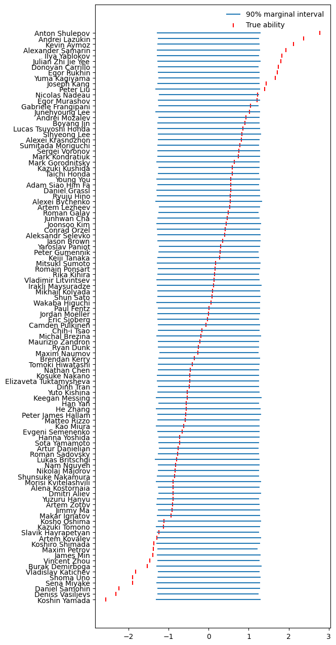
Simulated data ability priors
This seemed more or less fine.
Next I made a prior predictive check, comparing each observed score with the distribution of modelled scores:
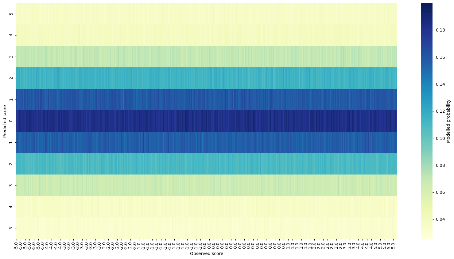
Simulated data prior predictive checks
Again nothing especially worrying, at least at this early stage.
Repeating the same plots for the fitted data gave these results:
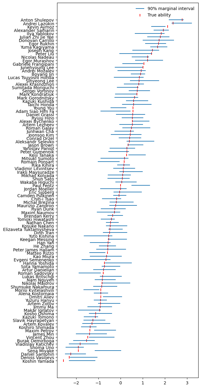
Simulated data ability posteriors
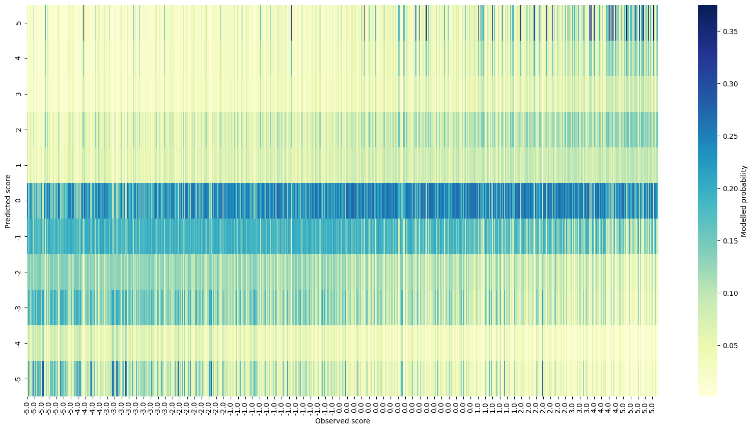
Simulated data posterior predictive checks
It’s nice that the available data seems sufficient to separate the skaters quite cleanly and that there is a visible, albeit not the sharpest, relationship between the observed outcome and the model’s predictions. The next logical step was to see how the model predicts some real data.
Fitting real data
Again the fitting and loo results were ok, but with a warning for the prior model:
Loo comparison:
                                            rank          loo        p_loo       d_loo  ...         se       dse  warning
real_study-20210322173057-simple_posterior     0 -4409.900382    81.597118     0.00000  ...  39.440729   0.00000    False
real_study-20210322173057-simple_prior         1 -8289.477432  2487.627217  3879.57705  ...  44.615350  62.40983     True
The posterior predictive check shows a decent visual relationship between observed and predicted scores. It’s interesting that there seems to be a lot of mis-prediction for the low observed scores on the left compared to the high ones on the right.
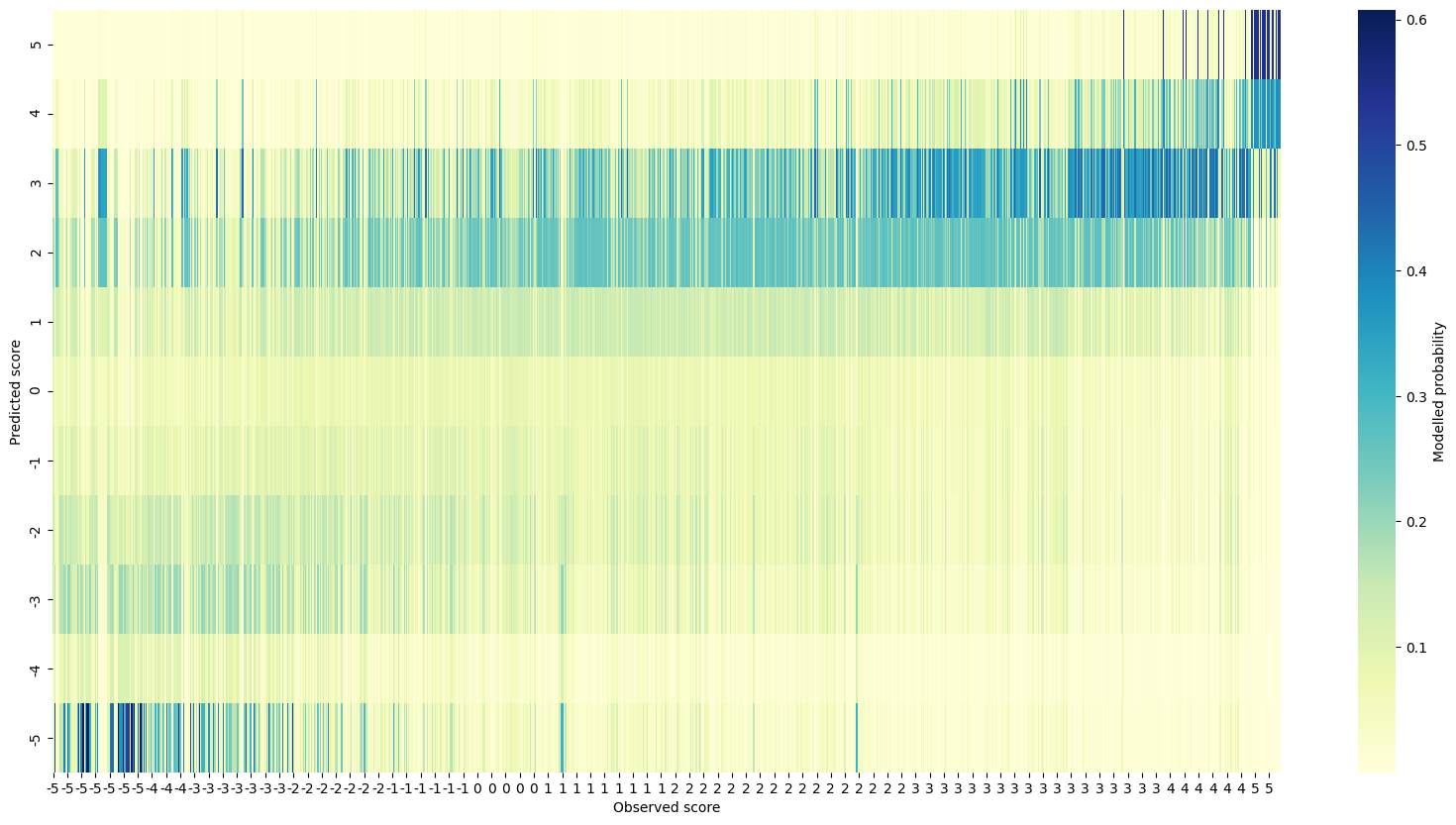
Real data posterior predictive checks
Finally, here are the modelled abilities, according to the real data:
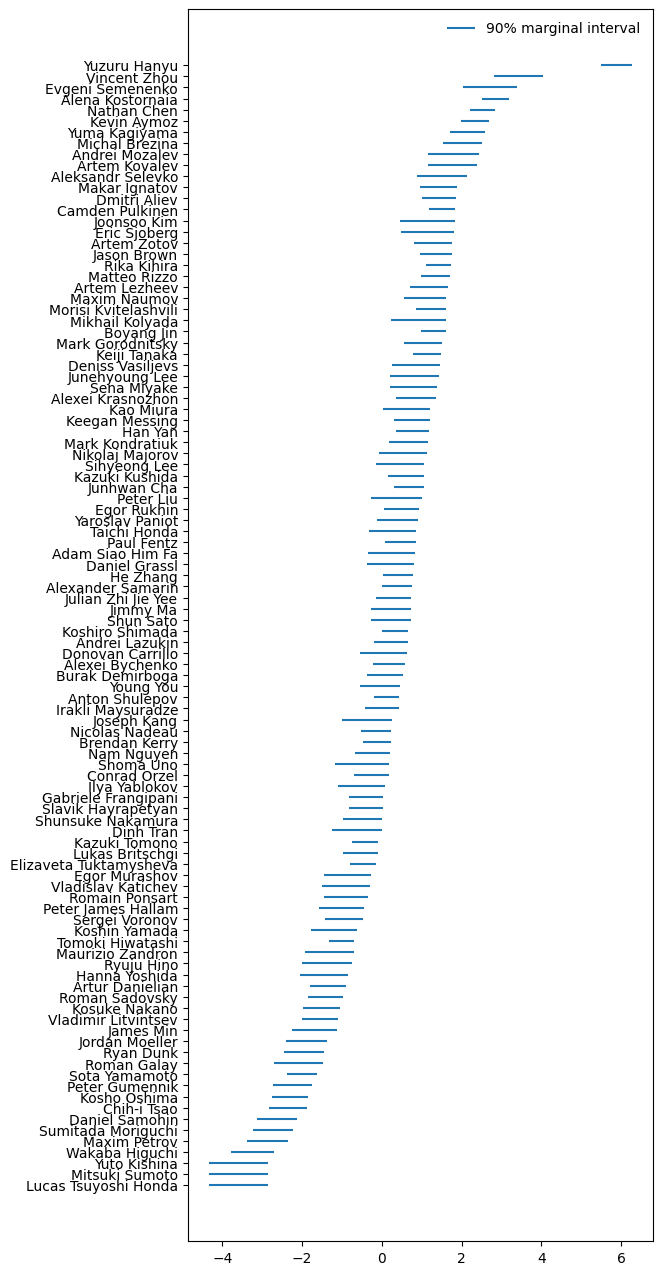
Real data ability posteriors
That’s right, the model’s answer to the title question is Yuzuru Hanyu, by a mile.

Conclusion
The model’s striking opinion about Yuzuru is defensible, as his triple axel is ridiculously good. This video showing how the jump has evolved through his career makes it clear how amazingly Yuzuru has been pulling it off in the last few seasons:
Still 5-6 standard deviations away from the average seems possibly a bit too extreme. Perhaps this is a clue as to how the model could be improved.
The next post in this series will attempt to do exactly that, comparing different models against the simple one.